Statistical Modeling with Mediator-outcome Confounders Affected by the Exposure
2022-03-30
Source:vignettes/post_exposure_confounding.Rmd
post_exposure_confounding.RmdThis example demonstrates how to use cmest when there are mediator-outcome confounders affected by the exposure. For this purpose, we simulate some data containing a continuous baseline confounder \(C_1\), a binary baseline confounder \(C_2\), a binary exposure \(A\), a continuous mediator-outcome confounder affected by the exposure \(L\), a binary mediator \(M\) and a binary outcome \(Y\). The true regression models for \(A\), \(L\), \(M\) and \(Y\) are: \[logit(E(A|C_1,C_2))=0.2+0.5C_1+0.1C_2\] \[E(L|A,C_1,C_2)=1+A-C_1-0.5C_2\] \[logit(E(M|A,L,C_1,C_2))=1+2A-L+1.5C_1+0.8C_2\] \[logit(E(Y|A,L,M,C_1,C_2)))=-3-0.4A-1.2M+0.5AM-0.5L+0.3C_1-0.6C_2\]
set.seed(1)
expit <- function(x) exp(x)/(1+exp(x))
n <- 10000
C1 <- rnorm(n, mean = 1, sd = 0.1)
C2 <- rbinom(n, 1, 0.6)
A <- rbinom(n, 1, expit(0.2 + 0.5*C1 + 0.1*C2))
L <- rnorm(n, mean = 1 + A - C1 - 0.5*C2, sd = 0.5)
M <- rbinom(n, 1, expit(1 + 2*A - L + 1.5*C1 + 0.8*C2))
Y <- rbinom(n, 1, expit(-3 - 0.4*A - 1.2*M + 0.5*A*M - 0.5*L + 0.3*C1 - 0.6*C2))
data <- data.frame(A, M, Y, C1, C2, L)
The DAG for this scientific setting is:
## Loading required package: dplyr##
## Attaching package: 'dplyr'## The following objects are masked from 'package:stats':
##
## filter, lag## The following objects are masked from 'package:base':
##
## intersect, setdiff, setequal, union## Loading required package: mstate## Loading required package: survival## Loading required package: tidyr
cmdag(outcome = "Y", exposure = "A", mediator = "M",
      basec = c("C1", "C2"), postc = "L", node = TRUE, text_col = "white")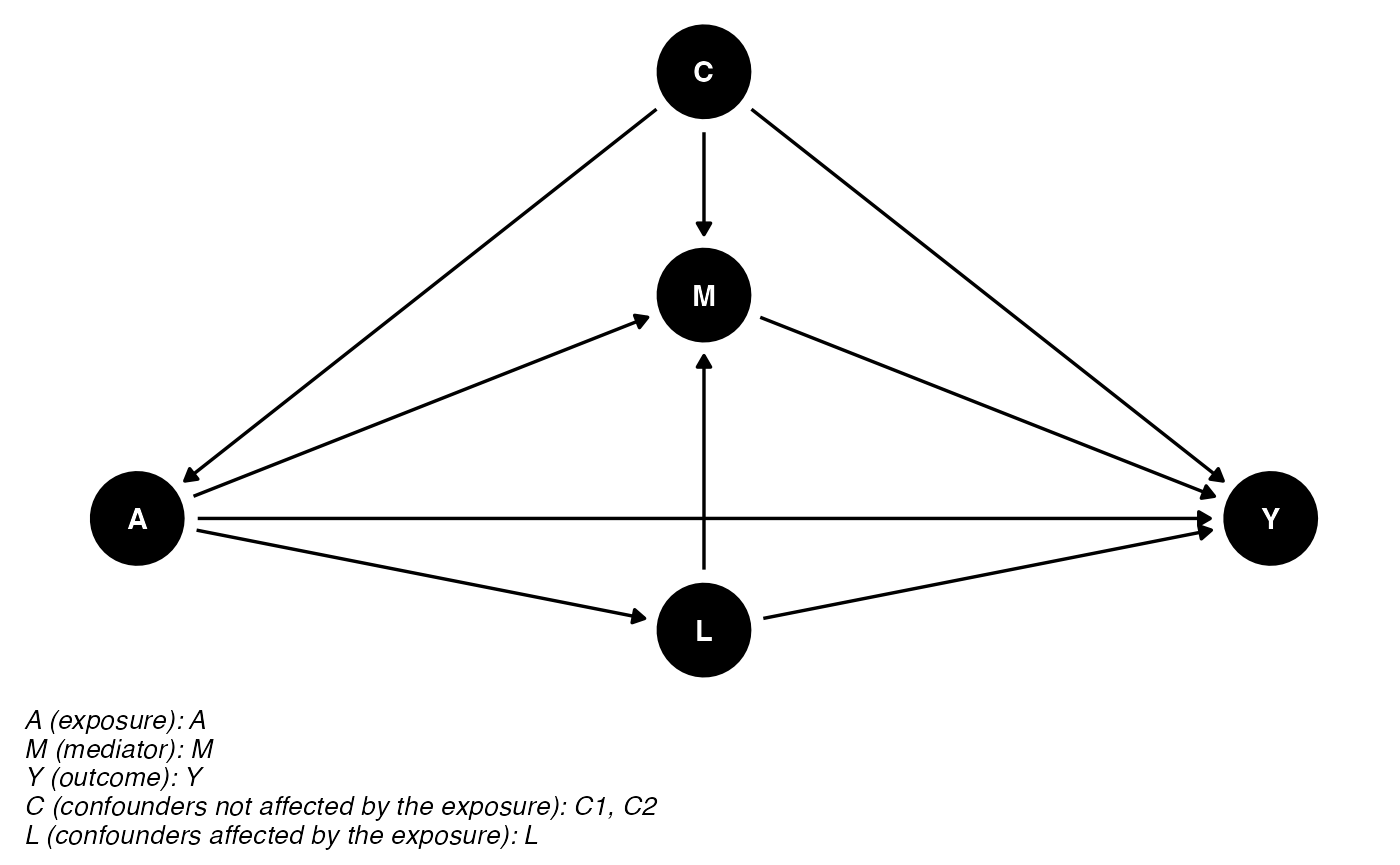
In this setting, we can use the marginal structural model and the \(g\)-formula approach. The results are shown below.
The Marginal Structural Model
res_msm <- cmest(data = data, model = "msm", outcome = "Y", exposure = "A",
                 mediator = "M", basec = c("C1", "C2"), postc = "L", EMint = TRUE,
                 ereg = "logistic", yreg = "logistic", mreg = list("logistic"),
                 wmnomreg = list("logistic"), wmdenomreg = list("logistic"),
                 astar = 0, a = 1, mval = list(1),
                 estimation = "imputation", inference = "bootstrap", nboot = 2)
summary(res_msm)## Causal Mediation Analysis
##
## # Outcome regression:
##
## Call:
## glm(formula = Y ~ A + M + A * M, family = binomial(), data = getCall(x$reg.output$yreg)$data,
## weights = getCall(x$reg.output$yreg)$weights)
##
## Deviance Residuals:
## Min 1Q Median 3Q Max
## -0.6465 -0.1964 -0.1428 -0.1399 3.3658
##
## Coefficients:
## Estimate Std. Error z value Pr(>|z|)
## (Intercept) -3.49700 0.47457 -7.369 1.72e-13 ***
## A 0.09466 0.67862 0.139 0.889
## M -0.40808 0.49218 -0.829 0.407
## A:M -0.79067 0.70198 -1.126 0.260
## ---
## Signif. codes: 0 '***' 0.001 '**' 0.01 '*' 0.05 '.' 0.1 ' ' 1
##
## (Dispersion parameter for binomial family taken to be 1)
##
## Null deviance: 1432.5 on 9999 degrees of freedom
## Residual deviance: 1412.9 on 9996 degrees of freedom
## AIC: 1432.5
##
## Number of Fisher Scoring iterations: 7
##
##
## # Mediator regressions:
##
## Call:
## glm(formula = M ~ A, family = binomial(), data = getCall(x$reg.output$mreg[[1L]])$data,
## weights = getCall(x$reg.output$mreg[[1L]])$weights)
##
## Deviance Residuals:
## Min 1Q Median 3Q Max
## -2.9114 0.1972 0.1999 0.3089 0.3437
##
## Coefficients:
## Estimate Std. Error z value Pr(>|z|)
## (Intercept) 2.96393 0.08185 36.211 < 2e-16 ***
## A 0.95266 0.11992 7.944 1.95e-15 ***
## ---
## Signif. codes: 0 '***' 0.001 '**' 0.01 '*' 0.05 '.' 0.1 ' ' 1
##
## (Dispersion parameter for binomial family taken to be 1)
##
## Null deviance: 2623.2 on 9999 degrees of freedom
## Residual deviance: 2560.6 on 9998 degrees of freedom
## AIC: 2580.5
##
## Number of Fisher Scoring iterations: 6
##
##
## # Mediator regressions for weighting (denominator):
##
## Call:
## glm(formula = M ~ A + C1 + C2 + L, family = binomial(), data = getCall(x$reg.output$wmdenomreg[[1L]])$data,
## weights = getCall(x$reg.output$wmdenomreg[[1L]])$weights)
##
## Deviance Residuals:
## Min 1Q Median 3Q Max
## -3.4241 0.1334 0.1885 0.2668 0.8260
##
## Coefficients:
## Estimate Std. Error z value Pr(>|z|)
## (Intercept) 0.9946 0.6067 1.639 0.1012
## A 1.8884 0.1726 10.944 < 2e-16 ***
## C1 1.4955 0.6090 2.456 0.0141 *
## C2 0.8166 0.1410 5.793 6.92e-09 ***
## L -0.9171 0.1215 -7.546 4.50e-14 ***
## ---
## Signif. codes: 0 '***' 0.001 '**' 0.01 '*' 0.05 '.' 0.1 ' ' 1
##
## (Dispersion parameter for binomial family taken to be 1)
##
## Null deviance: 2646.0 on 9999 degrees of freedom
## Residual deviance: 2397.3 on 9995 degrees of freedom
## AIC: 2407.3
##
## Number of Fisher Scoring iterations: 7
##
##
## # Mediator regressions for weighting (nominator):
##
## Call:
## glm(formula = M ~ A, family = binomial(), data = getCall(x$reg.output$wmnomreg[[1L]])$data,
## weights = getCall(x$reg.output$wmnomreg[[1L]])$weights)
##
## Deviance Residuals:
## Min 1Q Median 3Q Max
## -2.8106 0.1972 0.1972 0.3224 0.3224
##
## Coefficients:
## Estimate Std. Error z value Pr(>|z|)
## (Intercept) 2.93070 0.08064 36.345 <2e-16 ***
## A 0.99963 0.11952 8.364 <2e-16 ***
## ---
## Signif. codes: 0 '***' 0.001 '**' 0.01 '*' 0.05 '.' 0.1 ' ' 1
##
## (Dispersion parameter for binomial family taken to be 1)
##
## Null deviance: 2646.0 on 9999 degrees of freedom
## Residual deviance: 2576.3 on 9998 degrees of freedom
## AIC: 2580.3
##
## Number of Fisher Scoring iterations: 6
##
##
## # Exposure regression for weighting:
##
## Call:
## glm(formula = A ~ C1 + C2, family = binomial(), data = getCall(x$reg.output$ereg)$data,
## weights = getCall(x$reg.output$ereg)$weights)
##
## Deviance Residuals:
## Min 1Q Median 3Q Max
## -1.6126 -1.4791 0.8573 0.8867 0.9750
##
## Coefficients:
## Estimate Std. Error z value Pr(>|z|)
## (Intercept) 0.08342 0.21440 0.389 0.69723
## C1 0.60899 0.21208 2.872 0.00409 **
## C2 0.10532 0.04375 2.407 0.01606 *
## ---
## Signif. codes: 0 '***' 0.001 '**' 0.01 '*' 0.05 '.' 0.1 ' ' 1
##
## (Dispersion parameter for binomial family taken to be 1)
##
## Null deviance: 12534 on 9999 degrees of freedom
## Residual deviance: 12520 on 9997 degrees of freedom
## AIC: 12526
##
## Number of Fisher Scoring iterations: 4
##
##
## # Effect decomposition on the risk ratio scale via the marginal structural model
##
## Direct counterfactual imputation estimation with
## bootstrap standard errors, percentile confidence intervals and p-values
##
## Estimate Std.error 95% CIL 95% CIU P.val
## Rcde 0.5035510 0.1696963 0.3942646 0.622 <2e-16 ***
## rRpnde 0.5444178 0.1812002 0.4051440 0.648 <2e-16 ***
## rRtnde 0.5208059 0.1743300 0.3991930 0.633 <2e-16 ***
## rRpnie 0.9867847 0.0087895 1.0023348 1.014 <2e-16 ***
## rRtnie 0.9439869 0.0151504 0.9788925 0.999 <2e-16 ***
## Rte 0.5139232 0.1712168 0.4048390 0.635 <2e-16 ***
## ERcde -0.4852025 0.1803464 -0.6204261 -0.378 <2e-16 ***
## rERintref 0.0296203 0.0008538 0.0269944 0.028 <2e-16 ***
## rERintmed -0.0172792 0.0011939 -0.0161869 -0.015 <2e-16 ***
## rERpnie -0.0132153 0.0087895 0.0023366 0.014 <2e-16 ***
## ERcde(prop) 0.9982014 0.0040755 1.0391856 1.045 <2e-16 ***
## rERintref(prop) -0.0609374 0.0238952 -0.0778943 -0.046 <2e-16 ***
## rERintmed(prop) 0.0355483 0.0149357 0.0247657 0.045 <2e-16 ***
## rERpnie(prop) 0.0271878 0.0130350 -0.0236356 -0.006 <2e-16 ***
## rpm 0.0627361 0.0279707 0.0011300 0.039 <2e-16 ***
## rint -0.0253891 0.0089595 -0.0330625 -0.021 <2e-16 ***
## rpe 0.0017986 0.0040755 -0.0446609 -0.039 <2e-16 ***
## ---
## Signif. codes: 0 '***' 0.001 '**' 0.01 '*' 0.05 '.' 0.1 ' ' 1
##
## (Rcde: controlled direct effect risk ratio; rRpnde: randomized analogue of pure natural direct effect risk ratio; rRtnde: randomized analogue of total natural direct effect risk ratio; rRpnie: randomized analogue of pure natural indirect effect risk ratio; rRtnie: randomized analogue of total natural indirect effect risk ratio; Rte: total effect risk ratio; ERcde: excess relative risk due to controlled direct effect; rERintref: randomized analogue of excess relative risk due to reference interaction; rERintmed: randomized analogue of excess relative risk due to mediated interaction; rERpnie: randomized analogue of excess relative risk due to pure natural indirect effect; ERcde(prop): proportion ERcde; rERintref(prop): proportion rERintref; rERintmed(prop): proportion rERintmed; rERpnie(prop): proportion rERpnie; rpm: randomized analogue of overall proportion mediated; rint: randomized analogue of overall proportion attributable to interaction; rpe: randomized analogue of overall proportion eliminated)
##
## Relevant variable values:
## $a
## [1] 1
##
## $astar
## [1] 0
##
## $yval
## [1] "1"
##
## $mval
## $mval[[1]]
## [1] 1The g-formula Approach
res_gformula <- cmest(data = data, model = "gformula", outcome = "Y", exposure = "A",
                      mediator = "M", basec = c("C1", "C2"), postc = "L", EMint = TRUE,
                      mreg = list("logistic"), yreg = "logistic", postcreg = list("linear"),
                      astar = 0, a = 1, mval = list(1),
                      estimation = "imputation", inference = "bootstrap", nboot = 2)
summary(res_gformula)## Causal Mediation Analysis
##
## # Outcome regression:
##
## Call:
## glm(formula = Y ~ A + M + A * M + C1 + C2 + L, family = binomial(),
## data = getCall(x$reg.output$yreg)$data, weights = getCall(x$reg.output$yreg)$weights)
##
## Deviance Residuals:
## Min 1Q Median 3Q Max
## -0.3617 -0.1788 -0.1545 -0.1289 3.1833
##
## Coefficients:
## Estimate Std. Error z value Pr(>|z|)
## (Intercept) -2.7488 0.9365 -2.935 0.00333 **
## A -0.1267 0.6617 -0.192 0.84812
## M -0.7274 0.4136 -1.759 0.07863 .
## C1 -0.1906 0.8705 -0.219 0.82664
## C2 -0.5566 0.1933 -2.880 0.00397 **
## L -0.2242 0.1709 -1.312 0.18964
## A:M -0.3425 0.6635 -0.516 0.60572
## ---
## Signif. codes: 0 '***' 0.001 '**' 0.01 '*' 0.05 '.' 0.1 ' ' 1
##
## (Dispersion parameter for binomial family taken to be 1)
##
## Null deviance: 1447.7 on 9999 degrees of freedom
## Residual deviance: 1415.5 on 9993 degrees of freedom
## AIC: 1429.5
##
## Number of Fisher Scoring iterations: 7
##
##
## # Mediator regressions:
##
## Call:
## glm(formula = M ~ A + C1 + C2 + L, family = binomial(), data = getCall(x$reg.output$mreg[[1L]])$data,
## weights = getCall(x$reg.output$mreg[[1L]])$weights)
##
## Deviance Residuals:
## Min 1Q Median 3Q Max
## -3.4241 0.1334 0.1885 0.2668 0.8260
##
## Coefficients:
## Estimate Std. Error z value Pr(>|z|)
## (Intercept) 0.9946 0.6067 1.639 0.1012
## A 1.8884 0.1726 10.944 < 2e-16 ***
## C1 1.4955 0.6090 2.456 0.0141 *
## C2 0.8166 0.1410 5.793 6.92e-09 ***
## L -0.9171 0.1215 -7.546 4.50e-14 ***
## ---
## Signif. codes: 0 '***' 0.001 '**' 0.01 '*' 0.05 '.' 0.1 ' ' 1
##
## (Dispersion parameter for binomial family taken to be 1)
##
## Null deviance: 2646.0 on 9999 degrees of freedom
## Residual deviance: 2397.3 on 9995 degrees of freedom
## AIC: 2407.3
##
## Number of Fisher Scoring iterations: 7
##
##
## # Regressions for mediator-outcome confounders affected by the exposure:
##
## Call:
## glm(formula = L ~ A + C1 + C2, family = gaussian(), data = getCall(x$reg.output$postcreg[[1L]])$data,
## weights = getCall(x$reg.output$postcreg[[1L]])$weights)
##
## Deviance Residuals:
## Min 1Q Median 3Q Max
## -1.82456 -0.34194 0.00712 0.33751 1.82462
##
## Coefficients:
## Estimate Std. Error t value Pr(>|t|)
## (Intercept) 1.00268 0.05077 19.75 <2e-16 ***
## A 1.00202 0.01081 92.68 <2e-16 ***
## C1 -1.00369 0.04980 -20.15 <2e-16 ***
## C2 -0.49437 0.01032 -47.92 <2e-16 ***
## ---
## Signif. codes: 0 '***' 0.001 '**' 0.01 '*' 0.05 '.' 0.1 ' ' 1
##
## (Dispersion parameter for gaussian family taken to be 0.2539334)
##
## Null deviance: 5324.2 on 9999 degrees of freedom
## Residual deviance: 2538.3 on 9996 degrees of freedom
## AIC: 14678
##
## Number of Fisher Scoring iterations: 2
##
##
## # Effect decomposition on the risk ratio scale via the g-formula approach
##
## Direct counterfactual imputation estimation with
## bootstrap standard errors, percentile confidence intervals and p-values
##
## Estimate Std.error 95% CIL 95% CIU P.val
## Rcde 0.504938 0.003275 0.631908 0.636 <2e-16 ***
## rRpnde 0.524665 0.062186 0.545245 0.629 <2e-16 ***
## rRtnde 0.513482 0.026241 0.597452 0.633 <2e-16 ***
## rRpnie 0.972198 0.029936 0.941736 0.982 <2e-16 ***
## rRtnie 0.951478 0.032623 0.988079 1.032 1
## Rte 0.499207 0.043654 0.562642 0.621 <2e-16 ***
## ERcde -0.471286 0.012399 -0.350420 -0.334 <2e-16 ***
## rERintref -0.004050 0.074586 -0.120836 -0.021 <2e-16 ***
## rERintmed 0.002344 0.048468 0.010442 0.076 <2e-16 ***
## rERpnie -0.027802 0.029936 -0.058241 -0.018 <2e-16 ***
## ERcde(prop) 0.941078 0.120817 0.763855 0.926 <2e-16 ***
## rERintref(prop) 0.008087 0.165221 0.053557 0.276 <2e-16 ***
## rERintmed(prop) -0.004680 0.108147 -0.172266 -0.027 <2e-16 ***
## rERpnie(prop) 0.055515 0.063743 0.047240 0.133 <2e-16 ***
## rpm 0.050835 0.044404 -0.039387 0.020 1
## rint 0.003407 0.057073 0.026588 0.103 <2e-16 ***
## rpe 0.058922 0.120817 0.073828 0.236 <2e-16 ***
## ---
## Signif. codes: 0 '***' 0.001 '**' 0.01 '*' 0.05 '.' 0.1 ' ' 1
##
## (Rcde: controlled direct effect risk ratio; rRpnde: randomized analogue of pure natural direct effect risk ratio; rRtnde: randomized analogue of total natural direct effect risk ratio; rRpnie: randomized analogue of pure natural indirect effect risk ratio; rRtnie: randomized analogue of total natural indirect effect risk ratio; Rte: total effect risk ratio; ERcde: excess relative risk due to controlled direct effect; rERintref: randomized analogue of excess relative risk due to reference interaction; rERintmed: randomized analogue of excess relative risk due to mediated interaction; rERpnie: randomized analogue of excess relative risk due to pure natural indirect effect; ERcde(prop): proportion ERcde; rERintref(prop): proportion rERintref; rERintmed(prop): proportion rERintmed; rERpnie(prop): proportion rERpnie; rpm: randomized analogue of overall proportion mediated; rint: randomized analogue of overall proportion attributable to interaction; rpe: randomized analogue of overall proportion eliminated)
##
## Relevant variable values:
## $a
## [1] 1
##
## $astar
## [1] 0
##
## $yval
## [1] "1"
##
## $mval
## $mval[[1]]
## [1] 1