Statistical Modeling with Multiple Mediators
2022-03-30
Source:vignettes/multiple_mediators.Rmd
multiple_mediators.RmdThis example demonstrates how to use cmest when there are multiple mediators. For this purpose, we simulate some data containing a continuous baseline confounder \(C_1\), a binary baseline confounder \(C_2\), a binary exposure \(A\), a count mediator \(M_1\), a categorical mediator \(M_2\) and a binary outcome \(Y\). The true regression models for \(A\), \(M_1\), \(M_2\) and \(Y\) are: \[logit(E(A|C_1,C_2))=0.2+0.5C_1+0.1C_2\] \[log(E(M_1|A,C_1,C_2))=1-2A+0.5C_1+0.8C_2\] \[log\frac{E[M_2=1|A,M_1,C_1,C_2]}{E[M_2=0|A,M_1,C_1,C_2]}=0.1+0.1A+0.4M_1-0.5C_1+0.1C_2\] \[log\frac{E[M_2=2|A,M_1,C_1,C_2]}{E[M_2=0|A,M_1,C_1,C_2]}=0.4+0.2A-0.1M_1-C_1+0.5C_2\] \[logit(E(Y|A,M_1,M_2,C_1,C_2)))=-4+0.8A-1.8M_1+0.5(M_2==1)+0.8(M_2==2)+0.5AM_1-0.4A(M_2==1)-1.4A(M_2==2)+0.3*C_1-0.6C_2\]
set.seed(1)
expit <- function(x) exp(x)/(1+exp(x))
n <- 10000
C1 <- rnorm(n, mean = 1, sd = 0.1)
C2 <- rbinom(n, 1, 0.6)
A <- rbinom(n, 1, expit(0.2 + 0.5*C1 + 0.1*C2))
M1 <- rpois(n, exp(1 - 2*A + 0.5*C1 + 0.8*C2))
linpred1 <- 0.1 + 0.1*A + 0.4*M1 - 0.5*C1 + 0.1*C2
linpred2 <- 0.4 + 0.2*A - 0.1*M1 - C1 + 0.5*C2
probm0 = 1 / (1 + exp(linpred1) + exp(linpred2))
probm1 = exp(linpred1) / (1 + exp(linpred1) + exp(linpred2))
probm2 = exp(linpred2) / (1 + exp(linpred1) + exp(linpred2))
M2 = factor(sapply(1:n, FUN = function(x) sample(c(0, 1, 2), size = 1, replace = TRUE,
                                                 prob=c(probm0[x],
                                                        probm1[x],
                                                        probm2[x]))))
Y <- rbinom(n, 1, expit(1 + 0.8*A - 1.8*M1 + 0.5*(M2 == 1) + 0.8*(M2 == 2) +
                          0.5*A*M1 - 0.4*A*(M2 == 1) - 1.4*A*(M2 == 2)  + 0.3*C1 - 0.6*C2))
data <- data.frame(A, M1, M2, Y, C1, C2)
The DAG for this scientific setting is:
## Loading required package: dplyr##
## Attaching package: 'dplyr'## The following objects are masked from 'package:stats':
##
## filter, lag## The following objects are masked from 'package:base':
##
## intersect, setdiff, setequal, union## Loading required package: mstate## Loading required package: survival## Loading required package: tidyr
cmdag(outcome = "Y", exposure = "A", mediator = c("M1", "M2"),
      basec = c("C1", "C2"), postc = NULL, node = TRUE, text_col = "white")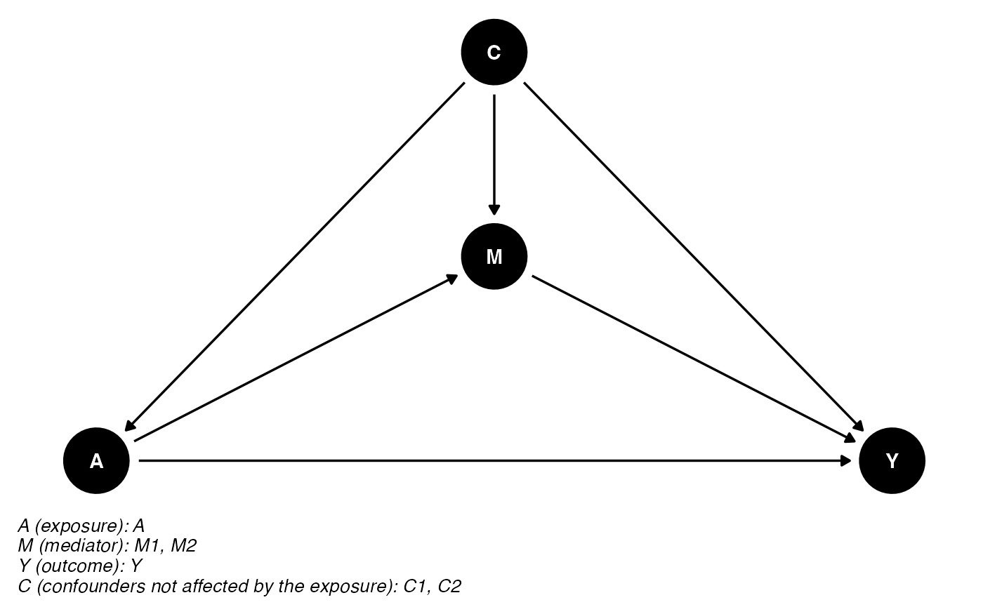
In this setting, we have a count mediator, so the marginal structural model is not available. We can use the rest five statistical modeling approaches. The results are shown below.
The Regression-based Approach
res_rb <- cmest(data = data, model = "rb", outcome = "Y", exposure = "A",
                mediator = c("M1", "M2"), basec = c("C1", "C2"), EMint = TRUE,
                mreg = list("poisson", "multinomial"), yreg = "logistic",
                astar = 0, a = 1, mval = list(0, 2),
                estimation = "imputation", inference = "bootstrap", nboot = 2)
summary(res_rb)## Causal Mediation Analysis
##
## # Outcome regression:
##
## Call:
## glm(formula = Y ~ A + M1 + M2 + A * M1 + A * M2 + C1 + C2, family = binomial(),
## data = getCall(x$reg.output$yreg)$data, weights = getCall(x$reg.output$yreg)$weights)
##
## Deviance Residuals:
## Min 1Q Median 3Q Max
## -2.2066 -0.5055 -0.0007 0.6383 3.3715
##
## Coefficients:
## Estimate Std. Error z value Pr(>|z|)
## (Intercept) 1.125104 0.478893 2.349 0.018804 *
## A 0.460265 0.400463 1.149 0.250419
## M1 -1.809307 0.180027 -10.050 < 2e-16 ***
## M21 -0.007101 0.364067 -0.020 0.984438
## M22 0.841167 0.405154 2.076 0.037879 *
## C1 0.504243 0.284671 1.771 0.076508 .
## C2 -0.643001 0.062025 -10.367 < 2e-16 ***
## A:M1 0.535812 0.183808 2.915 0.003556 **
## A:M21 0.129896 0.370967 0.350 0.726222
## A:M22 -1.447096 0.412172 -3.511 0.000447 ***
## ---
## Signif. codes: 0 '***' 0.001 '**' 0.01 '*' 0.05 '.' 0.1 ' ' 1
##
## (Dispersion parameter for binomial family taken to be 1)
##
## Null deviance: 13336.6 on 9999 degrees of freedom
## Residual deviance: 7347.9 on 9990 degrees of freedom
## AIC: 7367.9
##
## Number of Fisher Scoring iterations: 10
##
##
## # Mediator regressions:
##
## Call:
## glm(formula = M1 ~ A + C1 + C2, family = poisson(), data = getCall(x$reg.output$mreg[[1L]])$data,
## weights = getCall(x$reg.output$mreg[[1L]])$weights)
##
## Deviance Residuals:
## Min 1Q Median 3Q Max
## -3.4516 -1.0946 -0.2769 0.5079 3.4944
##
## Coefficients:
## Estimate Std. Error z value Pr(>|z|)
## (Intercept) 1.06240 0.05631 18.868 < 2e-16 ***
## A -2.00634 0.01331 -150.709 < 2e-16 ***
## C1 0.45102 0.05496 8.206 2.29e-16 ***
## C2 0.80084 0.01314 60.961 < 2e-16 ***
## ---
## Signif. codes: 0 '***' 0.001 '**' 0.01 '*' 0.05 '.' 0.1 ' ' 1
##
## (Dispersion parameter for poisson family taken to be 1)
##
## Null deviance: 43205 on 9999 degrees of freedom
## Residual deviance: 10846 on 9996 degrees of freedom
## AIC: 33081
##
## Number of Fisher Scoring iterations: 5
##
##
## Call:
## nnet::multinom(formula = M2 ~ A + C1 + C2, data = getCall(x$reg.output$mreg[[2]])$data,
## trace = FALSE, weights = getCall(x$reg.output$mreg[[2]])$weights)
##
## Coefficients:
## (Intercept) A C1 C2
## 1 1.946698 -1.785773 -0.3220412 0.7256062
## 2 0.654218 0.688984 -1.7259629 0.4295399
##
## Std. Errors:
## (Intercept) A C1 C2
## 1 0.2620667 0.06393051 0.2550181 0.05235024
## 2 0.3129261 0.10149606 0.2996053 0.06106820
##
## Residual Deviance: 17966.15
## AIC: 17982.15
##
## # Effect decomposition on the risk ratio scale via the regression-based approach
##
## Direct counterfactual imputation estimation with
## bootstrap standard errors, percentile confidence intervals and p-values
##
## Estimate Std.error 95% CIL 95% CIU P.val
## Rcde 0.840859 0.046685 0.788612 0.851 <2e-16 ***
## Rpnde 2.540010 0.249404 2.203176 2.538 <2e-16 ***
## Rtnde 1.198066 0.147841 1.024302 1.223 <2e-16 ***
## Rpnie 22.289482 0.880313 22.434122 23.617 <2e-16 ***
## Rtnie 10.513453 0.127523 10.808614 10.980 <2e-16 ***
## Rte 26.704271 2.414681 24.190746 27.435 <2e-16 ***
## ERcde -6.683714 1.717727 -8.708034 -6.400 <2e-16 ***
## ERintref 8.223724 1.468323 7.939139 9.912 <2e-16 ***
## ERintmed 2.874780 3.045590 -0.625298 3.466 1
## ERpnie 21.289482 0.880313 21.434936 22.618 <2e-16 ***
## ERcde(prop) -0.260023 0.099297 -0.375913 -0.243 <2e-16 ***
## ERintref(prop) 0.319936 0.094601 0.300688 0.428 <2e-16 ***
## ERintmed(prop) 0.111841 0.117704 -0.027554 0.131 1
## ERpnie(prop) 0.828247 0.122399 0.811238 0.976 <2e-16 ***
## pm 0.940087 0.004695 0.941819 0.948 <2e-16 ***
## int 0.431777 0.023102 0.400231 0.431 <2e-16 ***
## pe 1.260023 0.099297 1.242507 1.376 <2e-16 ***
## ---
## Signif. codes: 0 '***' 0.001 '**' 0.01 '*' 0.05 '.' 0.1 ' ' 1
##
## (Rcde: controlled direct effect risk ratio; Rpnde: pure natural direct effect risk ratio; Rtnde: total natural direct effect risk ratio; Rpnie: pure natural indirect effect risk ratio; Rtnie: total natural indirect effect risk ratio; Rte: total effect risk ratio; ERcde: excess relative risk due to controlled direct effect; ERintref: excess relative risk due to reference interaction; ERintmed: excess relative risk due to mediated interaction; ERpnie: excess relative risk due to pure natural indirect effect; ERcde(prop): proportion ERcde; ERintref(prop): proportion ERintref; ERintmed(prop): proportion ERintmed; ERpnie(prop): proportion ERpnie; pm: overall proportion mediated; int: overall proportion attributable to interaction; pe: overall proportion eliminated)
##
## Relevant variable values:
## $a
## [1] 1
##
## $astar
## [1] 0
##
## $yval
## [1] "1"
##
## $mval
## $mval[[1]]
## [1] 0
##
## $mval[[2]]
## [1] 2The Weighting-based Approach
res_wb <- cmest(data = data, model = "wb", outcome = "Y", exposure = "A",
                mediator = c("M1", "M2"), basec = c("C1", "C2"), EMint = TRUE,
                ereg = "logistic", yreg = "logistic",
                astar = 0, a = 1, mval = list(0, 2),
                estimation = "imputation", inference = "bootstrap", nboot = 2)
summary(res_wb)## Causal Mediation Analysis
##
## # Outcome regression:
##
## Call:
## glm(formula = Y ~ A + M1 + M2 + A * M1 + A * M2 + C1 + C2, family = binomial(),
## data = getCall(x$reg.output$yreg)$data, weights = getCall(x$reg.output$yreg)$weights)
##
## Deviance Residuals:
## Min 1Q Median 3Q Max
## -2.2066 -0.5055 -0.0007 0.6383 3.3715
##
## Coefficients:
## Estimate Std. Error z value Pr(>|z|)
## (Intercept) 1.125104 0.478893 2.349 0.018804 *
## A 0.460265 0.400463 1.149 0.250419
## M1 -1.809307 0.180027 -10.050 < 2e-16 ***
## M21 -0.007101 0.364067 -0.020 0.984438
## M22 0.841167 0.405154 2.076 0.037879 *
## C1 0.504243 0.284671 1.771 0.076508 .
## C2 -0.643001 0.062025 -10.367 < 2e-16 ***
## A:M1 0.535812 0.183808 2.915 0.003556 **
## A:M21 0.129896 0.370967 0.350 0.726222
## A:M22 -1.447096 0.412172 -3.511 0.000447 ***
## ---
## Signif. codes: 0 '***' 0.001 '**' 0.01 '*' 0.05 '.' 0.1 ' ' 1
##
## (Dispersion parameter for binomial family taken to be 1)
##
## Null deviance: 13336.6 on 9999 degrees of freedom
## Residual deviance: 7347.9 on 9990 degrees of freedom
## AIC: 7367.9
##
## Number of Fisher Scoring iterations: 10
##
##
## # Exposure regression for weighting:
##
## Call:
## glm(formula = A ~ C1 + C2, family = binomial(), data = getCall(x$reg.output$ereg)$data,
## weights = getCall(x$reg.output$ereg)$weights)
##
## Deviance Residuals:
## Min 1Q Median 3Q Max
## -1.6126 -1.4791 0.8573 0.8867 0.9750
##
## Coefficients:
## Estimate Std. Error z value Pr(>|z|)
## (Intercept) 0.08342 0.21440 0.389 0.69723
## C1 0.60899 0.21208 2.872 0.00409 **
## C2 0.10532 0.04375 2.407 0.01606 *
## ---
## Signif. codes: 0 '***' 0.001 '**' 0.01 '*' 0.05 '.' 0.1 ' ' 1
##
## (Dispersion parameter for binomial family taken to be 1)
##
## Null deviance: 12534 on 9999 degrees of freedom
## Residual deviance: 12520 on 9997 degrees of freedom
## AIC: 12526
##
## Number of Fisher Scoring iterations: 4
##
##
## # Effect decomposition on the risk ratio scale via the weighting-based approach
##
## Direct counterfactual imputation estimation with
## bootstrap standard errors, percentile confidence intervals and p-values
##
## Estimate Std.error 95% CIL 95% CIU P.val
## Rcde 0.840859 0.001153 0.843270 0.845 <2e-16 ***
## Rpnde 2.184496 0.124689 2.056035 2.224 <2e-16 ***
## Rtnde 1.197960 0.017578 1.135918 1.160 <2e-16 ***
## Rpnie 20.345349 1.376126 18.331408 20.180 <2e-16 ***
## Rtnie 11.157227 0.294594 10.127728 10.524 <2e-16 ***
## Rte 24.372911 1.917943 20.822968 23.400 <2e-16 ***
## ERcde -6.150317 0.544402 -5.782384 -5.051 <2e-16 ***
## ERintref 7.334812 0.669092 6.107188 7.006 <2e-16 ***
## ERintmed 2.843066 0.417128 1.436970 1.997 <2e-16 ***
## ERpnie 19.345349 1.376126 17.333768 19.183 <2e-16 ***
## ERcde(prop) -0.263139 0.002492 -0.258089 -0.255 <2e-16 ***
## ERintref(prop) 0.313817 0.003497 0.308008 0.313 <2e-16 ***
## ERintmed(prop) 0.121639 0.012419 0.072417 0.089 <2e-16 ***
## ERpnie(prop) 0.827682 0.013425 0.856280 0.874 <2e-16 ***
## pm 0.949322 0.001005 0.945382 0.947 <2e-16 ***
## int 0.435456 0.015916 0.380425 0.402 <2e-16 ***
## pe 1.263139 0.002492 1.254741 1.258 <2e-16 ***
## ---
## Signif. codes: 0 '***' 0.001 '**' 0.01 '*' 0.05 '.' 0.1 ' ' 1
##
## (Rcde: controlled direct effect risk ratio; Rpnde: pure natural direct effect risk ratio; Rtnde: total natural direct effect risk ratio; Rpnie: pure natural indirect effect risk ratio; Rtnie: total natural indirect effect risk ratio; Rte: total effect risk ratio; ERcde: excess relative risk due to controlled direct effect; ERintref: excess relative risk due to reference interaction; ERintmed: excess relative risk due to mediated interaction; ERpnie: excess relative risk due to pure natural indirect effect; ERcde(prop): proportion ERcde; ERintref(prop): proportion ERintref; ERintmed(prop): proportion ERintmed; ERpnie(prop): proportion ERpnie; pm: overall proportion mediated; int: overall proportion attributable to interaction; pe: overall proportion eliminated)
##
## Relevant variable values:
## $a
## [1] 1
##
## $astar
## [1] 0
##
## $yval
## [1] "1"
##
## $mval
## $mval[[1]]
## [1] 0
##
## $mval[[2]]
## [1] 2The Inverse Odds-ratio Weighting Approach
res_iorw <- cmest(data = data, model = "iorw", outcome = "Y", exposure = "A",
                  mediator = c("M1", "M2"), basec = c("C1", "C2"), EMint = TRUE,
                  ereg = "logistic", yreg = "logistic",
                  astar = 0, a = 1, mval = list(0, 2),
                  estimation = "imputation", inference = "bootstrap", nboot = 2)
summary(res_iorw)## Causal Mediation Analysis
##
## # Outcome regression for the total effect:
##
## Call:
## glm(formula = Y ~ A + C1 + C2, family = binomial(), data = getCall(x$reg.output$yregTot)$data,
## weights = getCall(x$reg.output$yregTot)$weights)
##
## Deviance Residuals:
## Min 1Q Median 3Q Max
## -1.6731 -1.0673 -0.1524 0.7688 2.5278
##
## Coefficients:
## Estimate Std. Error z value Pr(>|z|)
## (Intercept) -2.9946 0.2726 -10.987 <2e-16 ***
## A 4.1997 0.1205 34.855 <2e-16 ***
## C1 -0.1306 0.2473 -0.528 0.597
## C2 -1.3288 0.0534 -24.885 <2e-16 ***
## ---
## Signif. codes: 0 '***' 0.001 '**' 0.01 '*' 0.05 '.' 0.1 ' ' 1
##
## (Dispersion parameter for binomial family taken to be 1)
##
## Null deviance: 13336.6 on 9999 degrees of freedom
## Residual deviance: 9397.2 on 9996 degrees of freedom
## AIC: 9405.2
##
## Number of Fisher Scoring iterations: 6
##
##
## # Outcome regression for the direct effect:
##
## Call:
## glm(formula = Y ~ A + C1 + C2, family = binomial(), data = getCall(x$reg.output$yregDir)$data,
## weights = getCall(x$reg.output$yregDir)$weights)
##
## Deviance Residuals:
## Min 1Q Median 3Q Max
## -4.7789 -0.0549 -0.0069 0.0818 8.4799
##
## Coefficients:
## Estimate Std. Error z value Pr(>|z|)
## (Intercept) -1.5600 0.7405 -2.107 0.0351 *
## A 1.7294 0.1460 11.848 <2e-16 ***
## C1 -1.2645 0.7413 -1.706 0.0880 .
## C2 -3.7661 0.4333 -8.691 <2e-16 ***
## ---
## Signif. codes: 0 '***' 0.001 '**' 0.01 '*' 0.05 '.' 0.1 ' ' 1
##
## (Dispersion parameter for binomial family taken to be 1)
##
## Null deviance: 1926.6 on 9999 degrees of freedom
## Residual deviance: 1423.0 on 9996 degrees of freedom
## AIC: 1214.1
##
## Number of Fisher Scoring iterations: 8
##
##
## # Exposure regression for weighting:
##
## Call:
## glm(formula = A ~ M1 + M2 + C1 + C2, family = binomial(), data = getCall(x$reg.output$ereg)$data,
## weights = getCall(x$reg.output$ereg)$weights)
##
## Deviance Residuals:
## Min 1Q Median 3Q Max
## -3.6520 -0.0024 0.0343 0.1447 3.1329
##
## Coefficients:
## Estimate Std. Error z value Pr(>|z|)
## (Intercept) 1.14163 0.58304 1.958 0.0502 .
## M1 -2.00321 0.05823 -34.402 < 2e-16 ***
## M21 0.08020 0.13700 0.585 0.5583
## M22 -0.01835 0.17781 -0.103 0.9178
## C1 3.43446 0.58316 5.889 3.88e-09 ***
## C2 4.84059 0.18684 25.907 < 2e-16 ***
## ---
## Signif. codes: 0 '***' 0.001 '**' 0.01 '*' 0.05 '.' 0.1 ' ' 1
##
## (Dispersion parameter for binomial family taken to be 1)
##
## Null deviance: 12534.4 on 9999 degrees of freedom
## Residual deviance: 2139.2 on 9994 degrees of freedom
## AIC: 2151.2
##
## Number of Fisher Scoring iterations: 8
##
##
## # Effect decomposition on the risk ratio scale via the inverse odds ratio weighting approach
##
## Direct counterfactual imputation estimation with
## bootstrap standard errors, percentile confidence intervals and p-values
##
## Estimate Std.error 95% CIL 95% CIU P.val
## Rte 23.713831 1.745561 24.962887 27.308 <2e-16 ***
## Rpnde 4.483896 0.448867 4.168979 4.772 <2e-16 ***
## Rtnie 5.288667 0.197403 5.722561 5.988 <2e-16 ***
## pm 0.846618 0.008286 0.856622 0.868 <2e-16 ***
## ---
## Signif. codes: 0 '***' 0.001 '**' 0.01 '*' 0.05 '.' 0.1 ' ' 1
##
## (Rte: total effect risk ratio; Rpnde: pure natural direct effect risk ratio; Rtnie: total natural indirect effect risk ratio; pm: proportion mediated)
##
## Relevant variable values:
## $a
## [1] 1
##
## $astar
## [1] 0
##
## $yval
## [1] "1"The Natural Effect Model
res_ne <- cmest(data = data, model = "ne", outcome = "Y", exposure = "A",
                mediator = c("M1", "M2"), basec = c("C1", "C2"), EMint = TRUE,
                yreg = "logistic",
                astar = 0, a = 1, mval = list(0, 2),
                estimation = "imputation", inference = "bootstrap", nboot = 2)
summary(res_ne)## Causal Mediation Analysis
##
## # Outcome regression:
##
## Call:
## glm(formula = Y ~ A + M1 + M2 + A * M1 + A * M2 + C1 + C2, family = binomial(),
## data = getCall(x$reg.output$yreg)$data, weights = getCall(x$reg.output$yreg)$weights)
##
## Deviance Residuals:
## Min 1Q Median 3Q Max
## -2.2066 -0.5055 -0.0007 0.6383 3.3715
##
## Coefficients:
## Estimate Std. Error z value Pr(>|z|)
## (Intercept) 1.125104 0.478893 2.349 0.018804 *
## A 0.460265 0.400463 1.149 0.250419
## M1 -1.809307 0.180027 -10.050 < 2e-16 ***
## M21 -0.007101 0.364067 -0.020 0.984438
## M22 0.841167 0.405154 2.076 0.037879 *
## C1 0.504243 0.284671 1.771 0.076508 .
## C2 -0.643001 0.062025 -10.367 < 2e-16 ***
## A:M1 0.535812 0.183808 2.915 0.003556 **
## A:M21 0.129896 0.370967 0.350 0.726222
## A:M22 -1.447096 0.412172 -3.511 0.000447 ***
## ---
## Signif. codes: 0 '***' 0.001 '**' 0.01 '*' 0.05 '.' 0.1 ' ' 1
##
## (Dispersion parameter for binomial family taken to be 1)
##
## Null deviance: 13336.6 on 9999 degrees of freedom
## Residual deviance: 7347.9 on 9990 degrees of freedom
## AIC: 7367.9
##
## Number of Fisher Scoring iterations: 10
##
##
##
## # Effect decomposition on the risk ratio scale via the natural effect model
##
## Direct counterfactual imputation estimation with
## bootstrap standard errors, percentile confidence intervals and p-values
##
## Estimate Std.error 95% CIL 95% CIU P.val
## Rcde 0.840859 0.086137 0.895442 1.011 1
## Rpnde 2.397002 0.104623 2.429955 2.571 <2e-16 ***
## Rtnde 1.212344 0.101779 1.330542 1.467 <2e-16 ***
## Rpnie 20.806505 1.917377 18.176285 20.752 <2e-16 ***
## Rtnie 10.523413 0.173974 10.741630 10.975 <2e-16 ***
## Rte 25.224641 0.701059 26.669640 27.612 <2e-16 ***
## ERcde -6.332043 3.477253 -4.288821 0.383 1
## ERintref 7.729045 3.581876 1.047182 5.859 <2e-16 ***
## ERintmed 3.021133 1.320940 5.284538 7.059 <2e-16 ***
## ERpnie 19.806505 1.917377 17.180793 19.757 <2e-16 ***
## ERcde(prop) -0.261389 0.131063 -0.160993 0.015 1
## ERintref(prop) 0.319057 0.133527 0.040616 0.220 <2e-16 ***
## ERintmed(prop) 0.124713 0.056884 0.198651 0.275 <2e-16 ***
## ERpnie(prop) 0.817618 0.054420 0.669220 0.742 <2e-16 ***
## pm 0.942331 0.002464 0.940984 0.944 <2e-16 ***
## int 0.443770 0.076643 0.315690 0.419 <2e-16 ***
## pe 1.261389 0.131063 0.984910 1.161 <2e-16 ***
## ---
## Signif. codes: 0 '***' 0.001 '**' 0.01 '*' 0.05 '.' 0.1 ' ' 1
##
## (Rcde: controlled direct effect risk ratio; Rpnde: pure natural direct effect risk ratio; Rtnde: total natural direct effect risk ratio; Rpnie: pure natural indirect effect risk ratio; Rtnie: total natural indirect effect risk ratio; Rte: total effect risk ratio; ERcde: excess relative risk due to controlled direct effect; ERintref: excess relative risk due to reference interaction; ERintmed: excess relative risk due to mediated interaction; ERpnie: excess relative risk due to pure natural indirect effect; ERcde(prop): proportion ERcde; ERintref(prop): proportion ERintref; ERintmed(prop): proportion ERintmed; ERpnie(prop): proportion ERpnie; pm: overall proportion mediated; int: overall proportion attributable to interaction; pe: overall proportion eliminated)
##
## Relevant variable values:
## $a
## [1] 1
##
## $astar
## [1] 0
##
## $yval
## [1] "1"
##
## $mval
## $mval[[1]]
## [1] 0
##
## $mval[[2]]
## [1] 2The g-formula Approach
res_gformula <- cmest(data = data, model = "gformula", outcome = "Y", exposure = "A",
                      mediator = c("M1", "M2"), basec = c("C1", "C2"), EMint = TRUE,
                      mreg = list("poisson", "multinomial"), yreg = "logistic",
                      astar = 0, a = 1, mval = list(0, 2),
                      estimation = "imputation", inference = "bootstrap", nboot = 2)
summary(res_gformula)## Causal Mediation Analysis
##
## # Outcome regression:
##
## Call:
## glm(formula = Y ~ A + M1 + M2 + A * M1 + A * M2 + C1 + C2, family = binomial(),
## data = getCall(x$reg.output$yreg)$data, weights = getCall(x$reg.output$yreg)$weights)
##
## Deviance Residuals:
## Min 1Q Median 3Q Max
## -2.2066 -0.5055 -0.0007 0.6383 3.3715
##
## Coefficients:
## Estimate Std. Error z value Pr(>|z|)
## (Intercept) 1.125104 0.478893 2.349 0.018804 *
## A 0.460265 0.400463 1.149 0.250419
## M1 -1.809307 0.180027 -10.050 < 2e-16 ***
## M21 -0.007101 0.364067 -0.020 0.984438
## M22 0.841167 0.405154 2.076 0.037879 *
## C1 0.504243 0.284671 1.771 0.076508 .
## C2 -0.643001 0.062025 -10.367 < 2e-16 ***
## A:M1 0.535812 0.183808 2.915 0.003556 **
## A:M21 0.129896 0.370967 0.350 0.726222
## A:M22 -1.447096 0.412172 -3.511 0.000447 ***
## ---
## Signif. codes: 0 '***' 0.001 '**' 0.01 '*' 0.05 '.' 0.1 ' ' 1
##
## (Dispersion parameter for binomial family taken to be 1)
##
## Null deviance: 13336.6 on 9999 degrees of freedom
## Residual deviance: 7347.9 on 9990 degrees of freedom
## AIC: 7367.9
##
## Number of Fisher Scoring iterations: 10
##
##
## # Mediator regressions:
##
## Call:
## glm(formula = M1 ~ A + C1 + C2, family = poisson(), data = getCall(x$reg.output$mreg[[1L]])$data,
## weights = getCall(x$reg.output$mreg[[1L]])$weights)
##
## Deviance Residuals:
## Min 1Q Median 3Q Max
## -3.4516 -1.0946 -0.2769 0.5079 3.4944
##
## Coefficients:
## Estimate Std. Error z value Pr(>|z|)
## (Intercept) 1.06240 0.05631 18.868 < 2e-16 ***
## A -2.00634 0.01331 -150.709 < 2e-16 ***
## C1 0.45102 0.05496 8.206 2.29e-16 ***
## C2 0.80084 0.01314 60.961 < 2e-16 ***
## ---
## Signif. codes: 0 '***' 0.001 '**' 0.01 '*' 0.05 '.' 0.1 ' ' 1
##
## (Dispersion parameter for poisson family taken to be 1)
##
## Null deviance: 43205 on 9999 degrees of freedom
## Residual deviance: 10846 on 9996 degrees of freedom
## AIC: 33081
##
## Number of Fisher Scoring iterations: 5
##
##
## Call:
## nnet::multinom(formula = M2 ~ A + C1 + C2, data = getCall(x$reg.output$mreg[[2]])$data,
## trace = FALSE, weights = getCall(x$reg.output$mreg[[2]])$weights)
##
## Coefficients:
## (Intercept) A C1 C2
## 1 1.946698 -1.785773 -0.3220412 0.7256062
## 2 0.654218 0.688984 -1.7259629 0.4295399
##
## Std. Errors:
## (Intercept) A C1 C2
## 1 0.2620667 0.06393051 0.2550181 0.05235024
## 2 0.3129261 0.10149606 0.2996053 0.06106820
##
## Residual Deviance: 17966.15
## AIC: 17982.15
##
## # Effect decomposition on the risk ratio scale via the g-formula approach
##
## Direct counterfactual imputation estimation with
## bootstrap standard errors, percentile confidence intervals and p-values
##
## Estimate Std.error 95% CIL 95% CIU P.val
## Rcde 0.840859 0.065592 0.771998 0.860 <2e-16 ***
## Rpnde 2.628791 0.301244 2.110514 2.515 <2e-16 ***
## Rtnde 1.206834 0.190209 1.003274 1.259 1
## Rpnie 23.580908 1.786324 22.156678 24.556 <2e-16 ***
## Rtnie 10.825600 0.435251 11.088659 11.673 <2e-16 ***
## Rte 28.458238 2.421510 24.636897 27.890 <2e-16 ***
## ERcde -7.113482 2.684539 -9.594347 -5.988 <2e-16 ***
## ERintref 8.742273 2.383294 7.503828 10.706 <2e-16 ***
## ERintmed 3.248539 3.906589 -1.029096 4.219 1
## ERpnie 22.580908 1.786324 21.159954 23.560 <2e-16 ***
## ERcde(prop) -0.259065 0.136412 -0.406495 -0.223 <2e-16 ***
## ERintref(prop) 0.318384 0.129441 0.279567 0.453 <2e-16 ***
## ERintmed(prop) 0.118308 0.149237 -0.044273 0.156 1
## ERpnie(prop) 0.822373 0.156208 0.787431 0.997 <2e-16 ***
## pm 0.940681 0.006971 0.943658 0.953 <2e-16 ***
## int 0.436693 0.019796 0.409198 0.436 <2e-16 ***
## pe 1.259065 0.136412 1.223225 1.406 <2e-16 ***
## ---
## Signif. codes: 0 '***' 0.001 '**' 0.01 '*' 0.05 '.' 0.1 ' ' 1
##
## (Rcde: controlled direct effect risk ratio; Rpnde: pure natural direct effect risk ratio; Rtnde: total natural direct effect risk ratio; Rpnie: pure natural indirect effect risk ratio; Rtnie: total natural indirect effect risk ratio; Rte: total effect risk ratio; ERcde: excess relative risk due to controlled direct effect; ERintref: excess relative risk due to reference interaction; ERintmed: excess relative risk due to mediated interaction; ERpnie: excess relative risk due to pure natural indirect effect; ERcde(prop): proportion ERcde; ERintref(prop): proportion ERintref; ERintmed(prop): proportion ERintmed; ERpnie(prop): proportion ERpnie; pm: overall proportion mediated; int: overall proportion attributable to interaction; pe: overall proportion eliminated)
##
## Relevant variable values:
## $a
## [1] 1
##
## $astar
## [1] 0
##
## $yval
## [1] "1"
##
## $mval
## $mval[[1]]
## [1] 0
##
## $mval[[2]]
## [1] 2