Multiple Imputations with Missing Data
2022-03-30
Source:vignettes/multiple_imputation.Rmd
multiple_imputation.RmdThis example demonstrates how to estimate causal effects with multiple imputations by using cmest when the dataset contains missing values. For this purpose, we simulate some data containing a continuous baseline confounder \(C_1\), a binary baseline confounder \(C_2\), a binary exposure \(A\), a binary mediator \(M\) and a binary outcome \(Y\). The true regression models for \(A\), \(M\) and \(Y\) are: \[logit(E(A|C_1,C_2))=0.2+0.5C_1+0.1C_2\] \[logit(E(M|A,C_1,C_2))=1+2A+1.5C_1+0.8C_2\] \[logit(E(Y|A,M,C_1,C_2)))=-3-0.4A-1.2M+0.5AM+0.3C_1-0.6C_2\]
To create the dataset with missing values, we randomly delete 10% of values in the dataset.
set.seed(1)
expit <- function(x) exp(x)/(1+exp(x))
n <- 10000
C1 <- rnorm(n, mean = 1, sd = 0.1)
C2 <- rbinom(n, 1, 0.6)
A <- rbinom(n, 1, expit(0.2 + 0.5*C1 + 0.1*C2))
M <- rbinom(n, 1, expit(1 + 2*A + 1.5*C1 + 0.8*C2))
Y <- rbinom(n, 1, expit(-3 - 0.4*A - 1.2*M + 0.5*A*M + 0.3*C1 - 0.6*C2))
data_noNA <- data.frame(A, M, Y, C1, C2)
missing <- sample(1:(5*n), n*0.1, replace = FALSE)
C1[missing[which(missing <= n)]] <- NA
C2[missing[which((missing > n)*(missing <= 2*n) == 1)] - n] <- NA
A[missing[which((missing > 2*n)*(missing <= 3*n) == 1)] - 2*n] <- NA
M[missing[which((missing > 3*n)*(missing <= 4*n) == 1)] - 3*n] <- NA
Y[missing[which((missing > 4*n)*(missing <= 5*n) == 1)] - 4*n] <- NA
data <- data.frame(A, M, Y, C1, C2)
The DAG for this scientific setting is:
## Loading required package: dplyr##
## Attaching package: 'dplyr'## The following objects are masked from 'package:stats':
##
## filter, lag## The following objects are masked from 'package:base':
##
## intersect, setdiff, setequal, union## Loading required package: mstate## Loading required package: survival## Loading required package: tidyr
cmdag(outcome = "Y", exposure = "A", mediator = "M",
      basec = c("C1", "C2"), postc = NULL, node = TRUE, text_col = "white")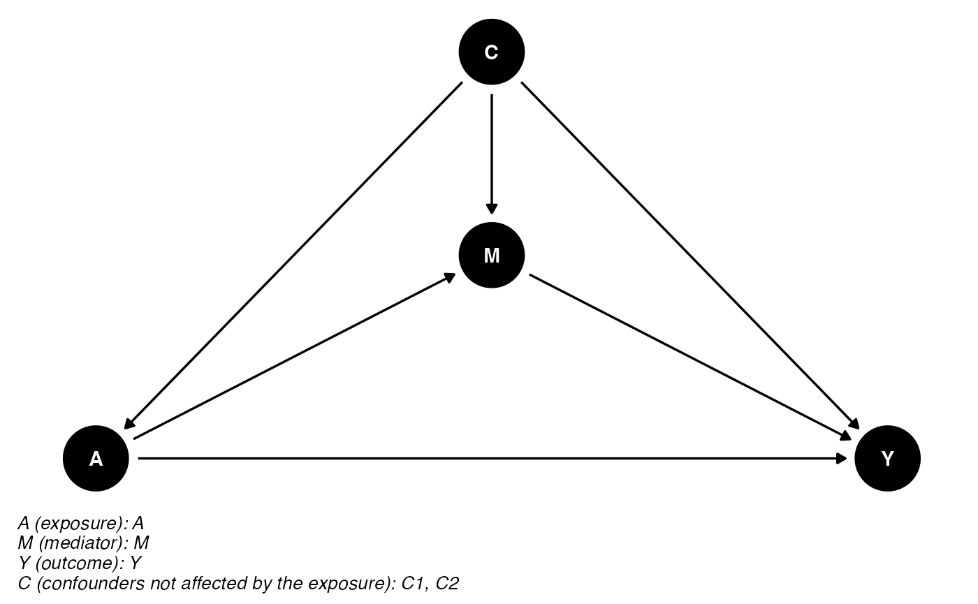
To conduct multiple imputations, we set the multimp argument to be TRUE. The regression-based approach is used for illustration. The multiple imputation results:
res_multimp <- cmest(data = data, model = "rb", outcome = "Y", exposure = "A",
                     mediator = "M", basec = c("C1", "C2"), EMint = TRUE,
                     mreg = list("logistic"), yreg = "logistic",
                     astar = 0, a = 1, mval = list(1),
                     estimation = "paramfunc", inference = "delta",
                     multimp = TRUE, m = 10)
summary(res_multimp)## Causal Mediation Analysis
##
## # Regressions with imputed dataset 1
##
## ## Outcome regression:
##
## Call:
## glm(formula = Y ~ A + M + A * M + C1 + C2, family = binomial(),
## data = getCall(x$reg.output[[1L]]$yreg)$data, weights = getCall(x$reg.output[[1L]]$yreg)$weights)
##
## Deviance Residuals:
## Min 1Q Median 3Q Max
## -0.5694 -0.2416 -0.1744 -0.1601 3.0488
##
## Coefficients:
## Estimate Std. Error z value Pr(>|z|)
## (Intercept) -3.6067 0.7610 -4.740 2.14e-06 ***
## A 0.6880 0.5286 1.301 0.19311
## M -1.0444 0.3732 -2.798 0.00514 **
## C1 0.9828 0.6875 1.429 0.15288
## C2 -0.8432 0.1443 -5.843 5.12e-09 ***
## A:M -0.4189 0.5542 -0.756 0.44969
## ---
## Signif. codes: 0 '***' 0.001 '**' 0.01 '*' 0.05 '.' 0.1 ' ' 1
##
## (Dispersion parameter for binomial family taken to be 1)
##
## Null deviance: 2030.4 on 9999 degrees of freedom
## Residual deviance: 1972.2 on 9994 degrees of freedom
## AIC: 1984.2
##
## Number of Fisher Scoring iterations: 7
##
##
## ## Mediator regressions:
##
## Call:
## glm(formula = M ~ A + C1 + C2, family = binomial(), data = getCall(x$reg.output[[1L]]$mreg[[1L]])$data,
## weights = getCall(x$reg.output[[1L]]$mreg[[1L]])$weights)
##
## Deviance Residuals:
## Min 1Q Median 3Q Max
## -3.2915 0.1100 0.1627 0.2428 0.5763
##
## Coefficients:
## Estimate Std. Error z value Pr(>|z|)
## (Intercept) 0.2134 0.6391 0.334 0.73848
## A 1.7157 0.1461 11.747 < 2e-16 ***
## C1 2.2136 0.6476 3.418 0.00063 ***
## C2 0.9837 0.1369 7.185 6.72e-13 ***
## ---
## Signif. codes: 0 '***' 0.001 '**' 0.01 '*' 0.05 '.' 0.1 ' ' 1
##
## (Dispersion parameter for binomial family taken to be 1)
##
## Null deviance: 2264.5 on 9999 degrees of freedom
## Residual deviance: 2034.0 on 9996 degrees of freedom
## AIC: 2042
##
## Number of Fisher Scoring iterations: 7
##
##
## # Regressions with imputed dataset 2
##
## ## Outcome regression:
##
## Call:
## glm(formula = Y ~ A + M + A * M + C1 + C2, family = binomial(),
## data = getCall(x$reg.output[[2L]]$yreg)$data, weights = getCall(x$reg.output[[2L]]$yreg)$weights)
##
## Deviance Residuals:
## Min 1Q Median 3Q Max
## -0.5675 -0.2408 -0.1734 -0.1610 3.0621
##
## Coefficients:
## Estimate Std. Error z value Pr(>|z|)
## (Intercept) -3.4557 0.7724 -4.474 7.67e-06 ***
## A 0.7235 0.5289 1.368 0.17129
## M -1.1024 0.3747 -2.942 0.00326 **
## C1 0.8216 0.7014 1.171 0.24143
## C2 -0.8368 0.1454 -5.753 8.75e-09 ***
## A:M -0.3930 0.5556 -0.707 0.47935
## ---
## Signif. codes: 0 '***' 0.001 '**' 0.01 '*' 0.05 '.' 0.1 ' ' 1
##
## (Dispersion parameter for binomial family taken to be 1)
##
## Null deviance: 1999.6 on 9999 degrees of freedom
## Residual deviance: 1941.7 on 9994 degrees of freedom
## AIC: 1953.7
##
## Number of Fisher Scoring iterations: 7
##
##
## ## Mediator regressions:
##
## Call:
## glm(formula = M ~ A + C1 + C2, family = binomial(), data = getCall(x$reg.output[[2L]]$mreg[[1L]])$data,
## weights = getCall(x$reg.output[[2L]]$mreg[[1L]])$weights)
##
## Deviance Residuals:
## Min 1Q Median 3Q Max
## -3.2872 0.1122 0.1581 0.2495 0.5865
##
## Coefficients:
## Estimate Std. Error z value Pr(>|z|)
## (Intercept) 0.06114 0.64423 0.095 0.924394
## A 1.74914 0.14643 11.945 < 2e-16 ***
## C1 2.38172 0.65266 3.649 0.000263 ***
## C2 0.89858 0.13520 6.646 3.01e-11 ***
## ---
## Signif. codes: 0 '***' 0.001 '**' 0.01 '*' 0.05 '.' 0.1 ' ' 1
##
## (Dispersion parameter for binomial family taken to be 1)
##
## Null deviance: 2279.3 on 9999 degrees of freedom
## Residual deviance: 2048.3 on 9996 degrees of freedom
## AIC: 2056.3
##
## Number of Fisher Scoring iterations: 7
##
##
## # Regressions with imputed dataset 3
##
## ## Outcome regression:
##
## Call:
## glm(formula = Y ~ A + M + A * M + C1 + C2, family = binomial(),
## data = getCall(x$reg.output[[3L]]$yreg)$data, weights = getCall(x$reg.output[[3L]]$yreg)$weights)
##
## Deviance Residuals:
## Min 1Q Median 3Q Max
## -0.5610 -0.2410 -0.1711 -0.1586 3.0539
##
## Coefficients:
## Estimate Std. Error z value Pr(>|z|)
## (Intercept) -3.4754 0.7762 -4.477 7.55e-06 ***
## A 0.6578 0.5285 1.245 0.21327
## M -1.0783 0.3738 -2.885 0.00391 **
## C1 0.8717 0.7056 1.235 0.21666
## C2 -0.8594 0.1457 -5.897 3.70e-09 ***
## A:M -0.3875 0.5546 -0.699 0.48473
## ---
## Signif. codes: 0 '***' 0.001 '**' 0.01 '*' 0.05 '.' 0.1 ' ' 1
##
## (Dispersion parameter for binomial family taken to be 1)
##
## Null deviance: 1999.6 on 9999 degrees of freedom
## Residual deviance: 1941.0 on 9994 degrees of freedom
## AIC: 1953
##
## Number of Fisher Scoring iterations: 7
##
##
## ## Mediator regressions:
##
## Call:
## glm(formula = M ~ A + C1 + C2, family = binomial(), data = getCall(x$reg.output[[3L]]$mreg[[1L]])$data,
## weights = getCall(x$reg.output[[3L]]$mreg[[1L]])$weights)
##
## Deviance Residuals:
## Min 1Q Median 3Q Max
## -3.2840 0.1135 0.1603 0.2463 0.5915
##
## Coefficients:
## Estimate Std. Error z value Pr(>|z|)
## (Intercept) -0.02469 0.64619 -0.038 0.969527
## A 1.70728 0.14525 11.754 < 2e-16 ***
## C1 2.48160 0.65504 3.788 0.000152 ***
## C2 0.90288 0.13534 6.671 2.53e-11 ***
## ---
## Signif. codes: 0 '***' 0.001 '**' 0.01 '*' 0.05 '.' 0.1 ' ' 1
##
## (Dispersion parameter for binomial family taken to be 1)
##
## Null deviance: 2271.9 on 9999 degrees of freedom
## Residual deviance: 2047.8 on 9996 degrees of freedom
## AIC: 2055.8
##
## Number of Fisher Scoring iterations: 7
##
##
## # Regressions with imputed dataset 4
##
## ## Outcome regression:
##
## Call:
## glm(formula = Y ~ A + M + A * M + C1 + C2, family = binomial(),
## data = getCall(x$reg.output[[4L]]$yreg)$data, weights = getCall(x$reg.output[[4L]]$yreg)$weights)
##
## Deviance Residuals:
## Min 1Q Median 3Q Max
## -0.6131 -0.2409 -0.1769 -0.1626 3.0550
##
## Coefficients:
## Estimate Std. Error z value Pr(>|z|)
## (Intercept) -3.5583 0.7664 -4.643 3.44e-06 ***
## A 0.8684 0.5120 1.696 0.08984 .
## M -1.0941 0.3742 -2.924 0.00346 **
## C1 0.9264 0.6936 1.336 0.18167
## C2 -0.8117 0.1435 -5.655 1.56e-08 ***
## A:M -0.5374 0.5389 -0.997 0.31868
## ---
## Signif. codes: 0 '***' 0.001 '**' 0.01 '*' 0.05 '.' 0.1 ' ' 1
##
## (Dispersion parameter for binomial family taken to be 1)
##
## Null deviance: 2038.1 on 9999 degrees of freedom
## Residual deviance: 1977.6 on 9994 degrees of freedom
## AIC: 1989.6
##
## Number of Fisher Scoring iterations: 7
##
##
## ## Mediator regressions:
##
## Call:
## glm(formula = M ~ A + C1 + C2, family = binomial(), data = getCall(x$reg.output[[4L]]$mreg[[1L]])$data,
## weights = getCall(x$reg.output[[4L]]$mreg[[1L]])$weights)
##
## Deviance Residuals:
## Min 1Q Median 3Q Max
## -3.2910 0.1110 0.1596 0.2461 0.5821
##
## Coefficients:
## Estimate Std. Error z value Pr(>|z|)
## (Intercept) 0.1220 0.6485 0.188 0.850782
## A 1.7418 0.1467 11.877 < 2e-16 ***
## C1 2.3162 0.6558 3.532 0.000413 ***
## C2 0.9316 0.1361 6.847 7.55e-12 ***
## ---
## Signif. codes: 0 '***' 0.001 '**' 0.01 '*' 0.05 '.' 0.1 ' ' 1
##
## (Dispersion parameter for binomial family taken to be 1)
##
## Null deviance: 2264.5 on 9999 degrees of freedom
## Residual deviance: 2035.6 on 9996 degrees of freedom
## AIC: 2043.6
##
## Number of Fisher Scoring iterations: 7
##
##
## # Regressions with imputed dataset 5
##
## ## Outcome regression:
##
## Call:
## glm(formula = Y ~ A + M + A * M + C1 + C2, family = binomial(),
## data = getCall(x$reg.output[[5L]]$yreg)$data, weights = getCall(x$reg.output[[5L]]$yreg)$weights)
##
## Deviance Residuals:
## Min 1Q Median 3Q Max
## -0.5628 -0.2464 -0.1719 -0.1620 3.0578
##
## Coefficients:
## Estimate Std. Error z value Pr(>|z|)
## (Intercept) -3.1670 0.7635 -4.148 3.35e-05 ***
## A 0.6129 0.5183 1.182 0.237047
## M -1.2113 0.3598 -3.367 0.000761 ***
## C1 0.6585 0.7005 0.940 0.347196
## C2 -0.8612 0.1449 -5.942 2.81e-09 ***
## A:M -0.2803 0.5454 -0.514 0.607333
## ---
## Signif. codes: 0 '***' 0.001 '**' 0.01 '*' 0.05 '.' 0.1 ' ' 1
##
## (Dispersion parameter for binomial family taken to be 1)
##
## Null deviance: 2015.0 on 9999 degrees of freedom
## Residual deviance: 1953.3 on 9994 degrees of freedom
## AIC: 1965.3
##
## Number of Fisher Scoring iterations: 7
##
##
## ## Mediator regressions:
##
## Call:
## glm(formula = M ~ A + C1 + C2, family = binomial(), data = getCall(x$reg.output[[5L]]$mreg[[1L]])$data,
## weights = getCall(x$reg.output[[5L]]$mreg[[1L]])$weights)
##
## Deviance Residuals:
## Min 1Q Median 3Q Max
## -3.2762 0.1129 0.1605 0.2487 0.5715
##
## Coefficients:
## Estimate Std. Error z value Pr(>|z|)
## (Intercept) 0.2134 0.6455 0.331 0.740950
## A 1.7214 0.1460 11.791 < 2e-16 ***
## C1 2.2401 0.6538 3.426 0.000612 ***
## C2 0.8976 0.1355 6.625 3.47e-11 ***
## ---
## Signif. codes: 0 '***' 0.001 '**' 0.01 '*' 0.05 '.' 0.1 ' ' 1
##
## (Dispersion parameter for binomial family taken to be 1)
##
## Null deviance: 2264.5 on 9999 degrees of freedom
## Residual deviance: 2041.5 on 9996 degrees of freedom
## AIC: 2049.5
##
## Number of Fisher Scoring iterations: 7
##
##
## # Effect decomposition on the risk ratio scale via the regression-based approach with multiple imputation
##
## Closed-form parameter function estimation with
## delta method standard errors, confidence intervals and p-values
##
## Estimate Std.error 95% CIL 95% CIU P.val
## Rcde 1.35895 0.23436 0.96919 1.905 0.0753 .
## Rpnde 1.44731 0.25058 1.03084 2.032 0.0327 *
## Rtnde 1.37654 0.23224 0.98896 1.916 0.0582 .
## Rpnie 0.92859 0.03747 0.85799 1.005 0.0663 .
## Rtnie 0.88318 0.05446 0.78264 0.997 0.0440 *
## Rte 1.27825 0.20622 0.93173 1.754 0.1281
## ERcde 0.32787 0.20880 -0.08137 0.737 0.1164
## ERintref 0.12035 0.12110 -0.11700 0.358 0.3203
## ERintmed -0.09812 0.09897 -0.29210 0.096 0.3215
## ERpnie -0.07139 0.03744 -0.14478 0.002 0.0566 .
## ERcde(prop) 1.17873 0.23528 0.71758 1.640 5.45e-07 ***
## ERintref(prop) 0.43179 0.47321 -0.49568 1.359 0.3615
## ERintmed(prop) -0.35192 0.38637 -1.10919 0.405 0.3624
## ERpnie(prop) -0.25861 0.23334 -0.71595 0.199 0.2677
## pm -0.61053 0.48589 -1.56286 0.342 0.2089
## int 0.07988 0.08780 -0.09220 0.252 0.3629
## pe -0.17873 0.23528 -0.63988 0.282 0.4475
## ---
## Signif. codes: 0 '***' 0.001 '**' 0.01 '*' 0.05 '.' 0.1 ' ' 1
##
## (Rcde: controlled direct effect risk ratio; Rpnde: pure natural direct effect risk ratio; Rtnde: total natural direct effect risk ratio; Rpnie: pure natural indirect effect risk ratio; Rtnie: total natural indirect effect risk ratio; Rte: total effect risk ratio; ERcde: excess relative risk due to controlled direct effect; ERintref: excess relative risk due to reference interaction; ERintmed: excess relative risk due to mediated interaction; ERpnie: excess relative risk due to pure natural indirect effect; ERcde(prop): proportion ERcde; ERintref(prop): proportion ERintref; ERintmed(prop): proportion ERintmed; ERpnie(prop): proportion ERpnie; pm: overall proportion mediated; int: overall proportion attributable to interaction; pe: overall proportion eliminated)
##
## Relevant variable values:
## $a
## [1] 1
##
## $astar
## [1] 0
##
## $yval
## [1] "1"
##
## $mval
## $mval[[1]]
## [1] 1
##
##
## $basecval
## $basecval[[1]]
## [1] 0.9993387
##
## $basecval[[2]]
## [1] 0.6060235Compare the multiple imputation results with true results:
res_noNA <- cmest(data = data_noNA, model = "rb", outcome = "Y", exposure = "A",
                  mediator = "M", basec = c("C1", "C2"), EMint = TRUE,
                  mreg = list("logistic"), yreg = "logistic",
                  astar = 0, a = 1, mval = list(1),
                  estimation = "paramfunc", inference = "delta")
summary(res_noNA)## Causal Mediation Analysis
##
## # Outcome regression:
##
## Call:
## glm(formula = Y ~ A + M + A * M + C1 + C2, family = binomial(),
## data = getCall(x$reg.output$yreg)$data, weights = getCall(x$reg.output$yreg)$weights)
##
## Deviance Residuals:
## Min 1Q Median 3Q Max
## -0.5681 -0.2414 -0.1741 -0.1604 3.0521
##
## Coefficients:
## Estimate Std. Error z value Pr(>|z|)
## (Intercept) -3.5731 0.7713 -4.633 3.61e-06 ***
## A 0.7084 0.5283 1.341 0.17990
## M -1.0471 0.3736 -2.803 0.00507 **
## C1 0.9337 0.6973 1.339 0.18054
## C2 -0.8415 0.1443 -5.829 5.56e-09 ***
## A:M -0.4222 0.5541 -0.762 0.44607
## ---
## Signif. codes: 0 '***' 0.001 '**' 0.01 '*' 0.05 '.' 0.1 ' ' 1
##
## (Dispersion parameter for binomial family taken to be 1)
##
## Null deviance: 2022.7 on 9999 degrees of freedom
## Residual deviance: 1965.0 on 9994 degrees of freedom
## AIC: 1977
##
## Number of Fisher Scoring iterations: 7
##
##
## # Mediator regressions:
##
## Call:
## glm(formula = M ~ A + C1 + C2, family = binomial(), data = getCall(x$reg.output$mreg[[1L]])$data,
## weights = getCall(x$reg.output$mreg[[1L]])$weights)
##
## Deviance Residuals:
## Min 1Q Median 3Q Max
## -3.2578 0.1145 0.1647 0.2519 0.5563
##
## Coefficients:
## Estimate Std. Error z value Pr(>|z|)
## (Intercept) 0.4353 0.6410 0.679 0.49712
## A 1.7076 0.1443 11.837 < 2e-16 ***
## C1 1.9982 0.6474 3.086 0.00203 **
## C2 0.9024 0.1345 6.709 1.96e-11 ***
## ---
## Signif. codes: 0 '***' 0.001 '**' 0.01 '*' 0.05 '.' 0.1 ' ' 1
##
## (Dispersion parameter for binomial family taken to be 1)
##
## Null deviance: 2294.0 on 9999 degrees of freedom
## Residual deviance: 2072.5 on 9996 degrees of freedom
## AIC: 2080.5
##
## Number of Fisher Scoring iterations: 7
##
##
## # Effect decomposition on the risk ratio scale via the regression-based approach
##
## Closed-form parameter function estimation with
## delta method standard errors, confidence intervals and p-values
##
## Estimate Std.error 95% CIL 95% CIU P.val
## Rcde 1.33138 0.22278 0.95912 1.848 0.0872 .
## Rpnde 1.41988 0.23708 1.02358 1.970 0.0358 *
## Rtnde 1.34928 0.22056 0.97940 1.859 0.0669 .
## Rpnie 0.93338 0.03576 0.86587 1.006 0.0719 .
## Rtnie 0.88697 0.05295 0.78902 0.997 0.0445 *
## Rte 1.25939 0.19804 0.92535 1.714 0.1425
## ERcde 0.30416 0.20019 -0.08820 0.697 0.1287
## ERintref 0.11571 0.11472 -0.10914 0.341 0.3131
## ERintmed -0.09387 0.09323 -0.27659 0.089 0.3140
## ERpnie -0.06662 0.03576 -0.13670 0.003 0.0624 .
## ERcde(prop) 1.17262 0.23540 0.71124 1.634 6.32e-07 ***
## ERintref(prop) 0.44610 0.49051 -0.51528 1.407 0.3631
## ERintmed(prop) -0.36189 0.39881 -1.14354 0.420 0.3642
## ERpnie(prop) -0.25684 0.23474 -0.71691 0.203 0.2739
## pm -0.61872 0.50289 -1.60437 0.367 0.2186
## int 0.08421 0.09264 -0.09736 0.266 0.3633
## pe -0.17262 0.23540 -0.63400 0.289 0.4634
## ---
## Signif. codes: 0 '***' 0.001 '**' 0.01 '*' 0.05 '.' 0.1 ' ' 1
##
## (Rcde: controlled direct effect risk ratio; Rpnde: pure natural direct effect risk ratio; Rtnde: total natural direct effect risk ratio; Rpnie: pure natural indirect effect risk ratio; Rtnie: total natural indirect effect risk ratio; Rte: total effect risk ratio; ERcde: excess relative risk due to controlled direct effect; ERintref: excess relative risk due to reference interaction; ERintmed: excess relative risk due to mediated interaction; ERpnie: excess relative risk due to pure natural indirect effect; ERcde(prop): proportion ERcde; ERintref(prop): proportion ERintref; ERintmed(prop): proportion ERintmed; ERpnie(prop): proportion ERpnie; pm: overall proportion mediated; int: overall proportion attributable to interaction; pe: overall proportion eliminated)
##
## Relevant variable values:
## $a
## [1] 1
##
## $astar
## [1] 0
##
## $yval
## [1] "1"
##
## $mval
## $mval[[1]]
## [1] 1
##
##
## $basecval
## $basecval[[1]]
## [1] 0.9993463
##
## $basecval[[2]]
## [1] 0.6061